| Guide for the DieCAST Ocean Model |
Modeled Oceanic Response and Sea Surface Cooling to Typhoon Kai-Tak
Yu-Heng Tseng, Sen Jan, David E. Dietrich, I-I Lin1, Ya-ting Chang, T. Y. Tang(2009), 'Modeled Oceanic Response and Sea Surface Cooling to Typhoon Kai-Tak', Terrestrial, Atmospheric and Oceanic Sciences (in press). (SCI)Abstract | ||||||||||||||
|
The ocean response to typhoon Kai-Tak is simulated using a fourth-order accurate, basin-scale ocean model. The surface winds of typhoon Kai-Tak were obtained from QuikSCAT satellite images blended with the ECMWF wind fields. An intense nonlinear mesoscale eddy is generated in the northeast South China Sea (SCS) with a Rossby number of O(1) and on a 50¡V100km horizontal scale. Inertial oscillation is clearly observed. Advection dominates as the strong wind shear drives the mixed layer flows outward, away from the typhoon center, thus forcing upwelling from deep levels with a high upwelling velocity (>30 m/day). A drop in sea surface temperature (SST) of more than 9¢XC is found in both observation and simulation. We attribute this significant SST drop to the influence of the slow moving typhoon, initial stratification and bathymetry-induced upwelling in the northeast of the SCS where the typhoon hovered. |
1. Introduction | ||||||||||||||
|
It is well known that tropical cyclones (TCs), also known as typhoons (in the Pacific) and hurricanes (in the Atlantic), draw their energy from warm ocean (Emanuel et al., 1986). Through air-sea interaction, ocean supplies energy for typhoon¡¦s intensification (Emanuel et al., 1986; Moon et al., 2007, 2008; Lin et al., 2009a). Pre-existing ocean mesoscale features and subsurface structures may be far more important than SST alone in the heat and moisture fluxes feeding the storm. Shay et al. (2000) noted an abrupt change in the intensity of hurricane Opal (9/28-10/5, 1995) when it passed over a large warm core eddy (WCE). Hurricane Katrina in August 2005 also showed a very similar intensification while passing over the Loop Current and WCE regions. Lin et al. (2005;2008) noted the critical role of warm ocean eddies in the western North Pacific category-5 typhoons in observing that 30% of these supertyphoons are fuelled by the warm ocean features. Wu et al. (2007) used simple coupled typhoon-ocean model to study the role of warm and cold eddies in typhoon¡¦s intensification. Typhoons also cause significant SST cooling which provides negative feedback to the overlying storm by weakening its intensity. For example, satellite images showed that SST dropped more than 9¢XC and 11¢XC in response to the passage of typhoons Kai-Tak (Lin et al., 2003) and Ling-Ling (Shang et al., 2008), respectively. Wu et al. (2008) studied the air¡Vsea interaction between typhoon Nari and the Kuroshio current using satellite observations and an ocean model. The intensity of typhoon Nari varied a few times when it crossed over the Kuroshio. These examples demonstrated the role of warm (cold) oceanic features in providing a positive (negative) feedback to the overlying storms by causing intensification (weakening) of the storms. In general, the primary mechanisms accounting for the sea surface cooling caused by TCs include mixed layer depth (vertical mixing/entrainment) and thermocline depth, exchange of air¡Vsea heat fluxes, and the storm¡¦s intensity and translation speed (Price, 1981; Lin et al., 2009b). Intense, slow moving typhoons usually cause a larger SST response. Since evaporation due to high winds over warm water sustains the thermodynamic cycle of a TC, SST cooling is thought to inhibit cyclone intensification, preventing the cyclones from attaining their potential intensity (Emanuel, 1999, 2001). When a typhoon encounters warm ocean features, SST cooling may be greatly suppressed primarily due to deep mixed-layer and thermocline depths (Wu et al., 2008). Early studies of upper-ocean response to TCs include field observations (e.g. Shay et al., 1989; Jacob et al., 2000) and three-dimensional numerical ocean models (Price, 1981; Price et al., 1994). Recent studies emphasized the understanding of the dynamic processes and interactions with the atmosphere, ocean heat content and ocean currents (e.g. Wu et al., 2008; Tsai et al., 2008; Oey et al., 2007; Sheng et al., 2007). Typically, the ocean¡¦s response to TCs can be divided into two stages: forced and relaxation stages. During the forced stage, the hurricane winds drive the mixed layer currents, causing SST cooling by vertical mixing (entrainment) and air¡Vsea heat exchange (e.g. loss of latent heat flux). The barotropic response consists of a non-geostrophic component which changes the sea surface height (a part of the inertia gravity response). The relaxation stage response follows a hurricane¡¦s passage, and is primarily influenced by inertial gravity oscillations excited by the TC. The mixed-layer velocity oscillates with a near-inertial period, and hence so too do the divergence and the associated upwelling and downwelling (Tsai et al., 2008). However, no study has focused on the causes and mechanisms of the significant temperature drops for particular TCs. Oceanic responses to TCs differ from one to another in several respects, and thereby make the processes difficult to study. This is further complicated by pre-existing oceanic features that modulate the upper ocean heat, mass and momentum balance due to advection. These mesoscale features need to be resolved in order to study the oceanic response. The extremely large amount of surface cooling in typhoon Kai-Tak was found mainly because of the continuous wind forced upwelling, a relatively shallow and warm mixed layer in the SCS and the local bathymetry of the SCS. The upwelling was enhanced by the typhoon¡¦s quasi-stationary motion. Similarly, a shallow mixed layer depth (~30 m) was also observed in the case of typhoon Ling-Ling and may have contributed to the 11¢XC temperature drop after its passage (Shang et al., 2008). The coastal upwelling and pre-existing ocean features significantly enhanced pronounced sea surface cooling. The main objectives of this paper are (1) to study the effect of a slow moving typhoon (Kai-Tak) in the South China Sea; (2) to quantify the physical processes which control the upper ocean thermal structure and strong surface cooling during the typhoon¡¦s passage; and (3) to assess the model¡¦s ability to reproduce the observed behavior of the oceanic responses to a typhoon without data assimilation. This paper is organized as follows: Section 2 describes the passage of typhoon Kai-Tak and relevant observations. Section 3 details the model configuration, initial and boundary conditions and model experiments. Section 4 compares the simulated results with observations followed by a qualitative description of the oceanic response to typhoon Kai-Tak. The mechanism that causes the significant SST drop is also investigated. The summary and conclusion are given in Section 5. ¡@ | ||||||||||||||
2. Typhoon Kai-Tak and Observations | ||||||||||||||
|
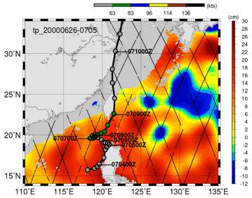
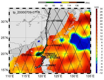
Typhoon Kai-Tak was declared a category 2 TC on the Saffir-Simpson hurricane scale. It lingered with slow speeds (0-1.4 m/s) in the northern SCS from July 5-8, 2000 before moving rapidly northwards thereafter (see Figure 1 for the storm track). The typhoon remained almost at rest during July 6-8. Remote sensed data provides an opportunity to investigate the surface behavior. Two remote sensed datasets were used in an earlier study (Lin et al., 2003); QuikSCAT and the Tropical Rainfall Measuring Mission (TRMM) Microwave Imager (TMI), respectively. The ocean surface wind vector (QuikSCAT) and the sea surface temperature (TMI) were measured day and night under both clear and cloudy conditions. The cloud penetrating capability of TMI allows the entire area of entrainment (location of a phytoplankton bloom patch) to be sensed. Here we have also incorporated QuikSCAT to provide an adequate wind forcing information in the model simulation. Figure 2 shows the daily averaged wind fields taken from QuikSCAT, illustrating how the typhoon lingered for several days in the northeast SCS during its passage of the SCS. More details about the wind forcing are provided in the next section. Before typhoon Kai-Tak¡¦s arrival, the SCS was characterized by predominantly warm SST greater than 30¢XC (Lin et al., 2003). Based on an average of ten-day TOPEX/Poseidon (T/P) satellite images, the Sea Surface Height Anomaly (SSHA) showed relatively calm eddy fields in the northeast SCS prior to July 5 (Figure 1(a)). The typhoon¡¦s strong winds (20-40 m/s) dominated the QuikSCAT wind field during July 7 to July 8 (Figure 2). Immediately after typhoon Kai-Tak¡¦s departure, a cold SST pool, with temperatures of 21.5-24¢XC (118-120¢XE, 19-20.5¢XN) of a size comparable to Kai-Tak¡¦s 150 km RMW (Radius of Maximum Wind), was observed and co-located with the typhoon¡¦s track. The minimum SST of 21.5¢XC was found at the center (118.9¢XE, 19.9¢XN) of the cold pool (Lin et al., 2003). In comparison with the pre-typhoon conditions, the SST had dropped by as much as 8-9¢XC. This cold pool slowly decayed after the passage of the typhoon, but still maintained a low temperature of 25¢XC. After the passage of typhoon Kai-Tak, the formation of a cyclonic eddy was observed, which is clearly intensified in the T/P image in Figure 1(b). The location, scale and peak of the growing cyclonic eddy (Figure 1(b)) matched well with the cold SST pool shown in Lin et al. (2003). The cyclonic eddy lasted for more than two weeks (Figure 1(b)). From these satellite images, the westward propagating Rossby waves and eddy fields in the North Pacific Ocean were identified while the cyclonic eddy grew in the northeast SCS. Some in-situ hydrographic surveys were conducted in the northeast SCS during the year 2000, including the South East Asia Time-series (SEATS) station (116¢XE, 18¢XN) in July 2000 and the Kuroshio Upstream Dynamics Experiment (KUDEX) mooring station KA1, labeled as red circular spot ¡§¡³¡¨ in Figure 2 (see Table 1 for detailed information). Both stations were under the influence of typhoon Kai-Tak. Some comparison with station KA1 will be discussed in Section 4. The initial stratification taken from the SEATS station (red diamond, ¡§¡º¡¨) is shown in Figure 2. The surface mixed layer, with a temperature of 29¢XC, was only about 20-30 m deep (Figure 2 bottom right). After the passage of typhoon Kai-Tak, the minimum temperature in the cold pool dropped to 21.6¢XC, which corresponded to the initial temperature at 71 m depth. The other station used in the comparison is an observation station at the southern tip of Taiwan (ST, labeled as a red square ¡§¡¼¡¨ in Figure 2).
| ||||||||||||||
| ||||||||||||||
| Figure 1: Ten-days averaged SSH TOPEX/Poseidon images before and after typhoon Kai-Tak (June 26-July5 (a) and July 9-July 18 (b), respectively) from the satellite showing the passage of typhoon Kai-Tak in northeast South China Sea. Luzon Strait is between Taiwan and Philippine. The storm-track of typhoon Kai-Tak is superimposed. | ||||||||||||||
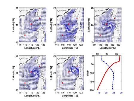 | ||||||||||||||
| Figure 2: Daily averaged QuikSCAT wind fields at 10 m from 7/3, 2000 (top left) to 7/7, 2000 (bottom center). The initial stratification (temperature and salinity) is shown in the bottom right panel, taken from the nearby SEAT station before the passage of Typhoon Kai-Tak. Observational stations: KA1 (o); SEAT (¡º); and ST (¡¼). | ||||||||||||||
3. Numerical Simulations | ||||||||||||||
| 3.1 Model setup and description
The Dual grid Pacific Ocean Model (DUPOM) used herein is based on the fourth-order accurate, collocated Arakawa-A grid DieCAST (Dietrich/Center for Air Sea Technology) model (Dietrich, 1997; Dietrich et al, 2004a; Tseng et al., 2005; Tseng and Breaker, 2007). The control volume equations include fluxes of the conservation properties (momentum, heat and salt) across control volume faces. The model domain covers the entire North Pacific Ocean, ranging from 30¢XS to 60¢XN and from 100¢XE to 80¢XW. To reduce the computational time, a dual grid approach was adopted based on a multiple grid framework, which uses higher resolutions to resolve eddies more realistically (Dietrich et al., 2008; Dietrich et al., 2004a). A 1/8¢X resolution was used west of 150¢XE, where a finer resolution was required to resolve the detailed Kuroshio Current and regional circulations, and a 1/4¢X resolution was used east of 150¢XE (Figure 3). The grids are fully two-way coupled at each coarser time step (time steps differ for the two grids) with a single coarse grid overlapping (i.e. 2¡Ñ2 in fine grid cells). The meander and eddy exchanges are seamless at the interface without inter-grid sponge layers or special treatments. Further details about the multiple grid approach can be found in Dietrich et al. (2008). Model bathymetry was interpolated from unfiltered ETOPO2 depth data, supplemented with the Taiwan National Center for Ocean Research 1 minute depth archive for the Asian seas. The vertical resolution is linear-exponentially stretched by 26 layers, with a 6-m thick top layer. Both grids share the same vertical grid. Within each grid, longitudinal resolution is uniform and latitudinal resolution is generated in such a manner that varying latitude and longitude grid increments are equal everywhere (Mercator grid). Simulation of mixed layer deepening and cooling during the typhoon¡¦s passage strongly depends on the choice of vertical mixing scheme. Except for vertical mixing parameters, the present model is very similar to the DieCAST model adaptation used to simulate the response to Hurricane Katrina (Dietrich, et al., 2007). Recent studies of upper ocean response to hurricanes, based on several bulk mixed layer entrainment schemes, have revealed significant differences in the heat and mass budgets (Jacob et al., 2000; Jacob and Shay, 2003; Prasad and Hogan, 2007). The suitability of any particular scheme is still subject to debate. Except for sub-grid scale vertical mixing parameters, the present model is very similar to that used by Sheng et al. (2006) and by Dietrich et al (2008). The model¡¦s sub-grid scale vertical mixing is parameterized by eddy diffusivity (for temperature and salinity) and viscosity (for momentum) using a modified Price (1981) scheme as described in Sheng et al. (2006). This new scheme, replacing the default Pacanowski and Philander (1982) scheme, was chosen to obtain a better mixed layer due to the strong wind forcing during the passage of the typhoon. Background lateral viscosity and diffusivity are 100 m²/s and 200 m²/s, respectively.The surface wind forcing in the basic model is obtained from the interpolated monthly Hellerman and Rosenstein winds (Hellerman and Rosenstein, 1983). The Levitus¡¦94 climatology (Levitus and Boyer, 1994) is used to initialize the model and to determine its surface sources of heat and fresh water (E-P) using the non-damping approach described in Dietrich et al. (2004b). The northern boundary is closed and the southern boundary condition (30¢XS) is slowly nudging toward climatology in a sponge layer. The bottom is insulated, with non slip conditions parameterized by a nonlinear bottom drag. Simulation of mixed layer deepening and cooling during the typhoon¡¦s passage strongly depends on the choice of vertical mixing scheme. Except for vertical mixing parameters, the present model is very similar to the DieCAST model adaptation used to simulate the response to Hurricane Katrina (Dietrich, et al., 2007). Recent studies of upper ocean response to hurricanes, based on several bulk mixed layer entrainment schemes, have revealed significant differences in the heat and mass budgets (Jacob et al., 2000; Jacob and Shay, 2003; Prasad and Hogan, 2007). The suitability of any particular scheme is still subject to debate. Except for sub-grid scale vertical mixing parameters, the present model is very similar to that used by Sheng et al. (2006) and by Dietrich et al (2008). The model¡¦s sub-grid scale vertical mixing is parameterized by eddy diffusivity (for temperature and salinity) and viscosity (for momentum) using a modified Price (1981) scheme as described in Sheng et al. (2006). This new scheme, replacing the default Pacanowski and Philander (1982) scheme, was chosen to obtain a better mixed layer due to the strong wind forcing during the passage of the typhoon. Background lateral viscosity and diffusivity are 100 m²/s and 200 m²/s, respectively. 3.2 Initial and boundary conditions The model was then driven by fields of 10 m wind stress extracted from six-hourly 2.5¢X ERA40. It is a well known fact that the ERA-40 product does not adequately resolve TCs. In this study, we further blended the ERA-40 winds with the QuikSCAT analyzed winds (Figure 2). Since the QuikSCAT data (twice per day) provided a more realistic and high quality wind field and may not be consistent with the ERA-40, a smoothing procedure was performed. We took the difference between the QuikSCAT and ERA-40 winds at each of the discrete observations and times. This difference was merged into an ¡§extended winds window¡¨ (EWW) grid, which was larger than the localized QuikSCAT wind field. The difference was then set to zero at the boundary of EWW, followed by a Poisson spreader to spread the difference between the QuikSCAT wind and the EWW grid boundaries. In order to minimize the nudging at the EWW grid boundaries, the EWW should extend laterally at least an eddy size beyond the QuikSCAT wind fields. Finally, the blended wind fields were then interpolated back to the model domain for application. Following Oey et al. (2006), the wind stress was calculated from the wind fields using a bulk formula:
where |ua| is wind speed (the maximum wind speed reached ~40 m/s from the QuikSCAT). This formula modifies Large and Pond (1981) to incorporate the limited drag coefficient for high wind speeds (Powell et al., 2003). All wind stresses were assumed to be in dynes/cm2 and of a magnitude less than 100 dynes/cm2. | ||||||||||||||
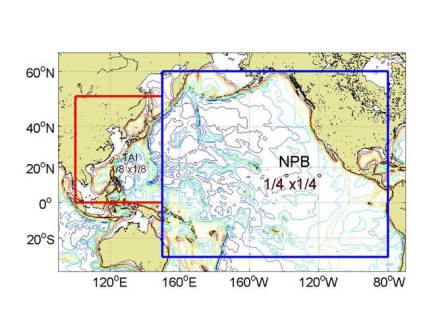 | ||||||||||||||
| Figure 3: The dual-grid Pacific Ocean Model, DUPOM, uses two grids in order to resolve critical features in Asia Marginal Sea, such as the Luzon Strait. ¡@ | ||||||||||||||
4. Numerical Results | ||||||||||||||
|
4.1 Typhoon-induced circulation and inertial currents during typhoon Kai-Tak
| ||||||||||||||
| ||||||||||||||
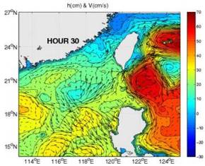
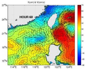
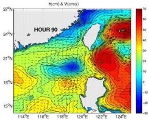
| Figure 4: Simulated surface current velocity and sea surface height (SSH) at different time. | ||||||||||||||
|
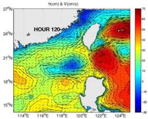
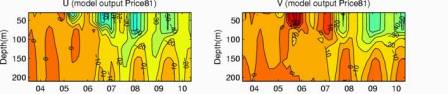
During the passage of typhoons, a sudden change of the surface wind stress can generate inertial motions in the upper ocean (Gill, 1982). In the north SCS, the averaged inertial period was about 35 hr (~20¢XN). The TC-induced inertial motions can last for two weeks or longer in some cases. We further compared the model velocities with those measured at the ADCP mooring station KA1 (KUDEX). The modeled zonal and meridional velocity (U and V, cm/s) components were compared with the observed velocity profiles vertically at the same location (Figure 5). To separate rapidly fluctuating inertial motions from other relatively low frequency inertial currents, a six hour low-pass filter was applied to the observed currents. Figure 5 shows the vertical profile comparison between the modeled and observed velocity components. The sensitivity of turbulent parameterization is also evaluated in the upper two panels. Both model and observation showed reasonably quasi-inertial oscillations ~34 hr. The model using the modified Price scheme showed more ordinary patterns, while the KA1 observation presented a larger variability. Using QuikSCAT wind vectors, entrainment-induced mixed layer deepening was estimated at ~100 m by a modified mixed layer turbulence parameterization (Sheng et al., 2006), and varied with time (Figure 5). This parameterization appears to perform relatively well compared with the traditional Pacanowski and Philander (1982), denoted by PP82 in the current simulation, due to the larger typhoon-induced vertical mixing and entrainment. The modeled mixed layer was shallower using the PP82 parameterization, resulting from insufficient vertical mixing in the surface mixed layer. More comparison between different turbulent parameterizations is discussed later. | ||||||||||||||
| ||||||||||||||
| Figure 5: Comparison of velocity profiles in the upper layer between the DUPOM and observation. Model (top), filtered observation (middle), observed raw data (bottom). | ||||||||||||||
|
Figure 6 shows additional time series velocity components in the upper layer at four different locations. The relative locations with respect to the typhoon center are west, east, north and south (top to bottom). Large inertial currents were concentrated around the typhoon. The flow velocities also changed directions during the passage of typhoon Kai-Tak. Unlike the wind-driven currents, the inertial amplitudes in a fast moving typhoon are usually much larger on the right of the typhoon path than on the left. This amplitude asymmetry is particularly striking when the wind vectors rotate at roughly the same rate as the inertial motion (Chang and Anthes 1978; Price 1981). It is found that the amplitude asymmetry is not so clear in Figure 6 due to the slow movement of typhoon Kai-Tak. It appears that the inertial currents were not destroyed by the quasi-stationary typhoon Kai-Tak. These inertial motions lasted for a long time after typhoon Kai-Tak had passed from the observation region (Chen, 2006). | ||||||||||||||
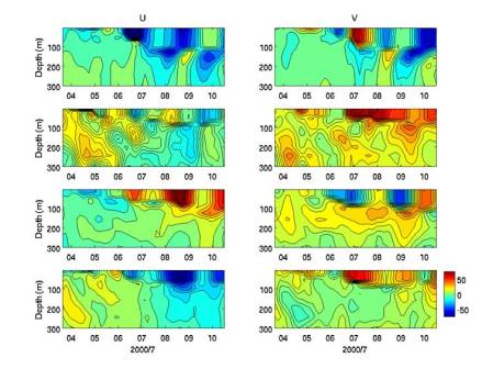 | ||||||||||||||
| Figure 6: Time-series velocity components in the upper layer at different locations. Relative locations with respect to typhoon center: west, east, north, south (from top to bottom). | ||||||||||||||
|
4.2 Sensitivity of turbulence parameterization
| ||||||||||||||
 (a) 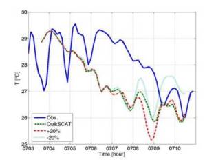 (b) | ||||||||||||||
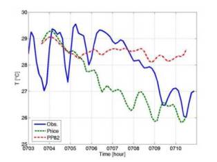
| Figure 7: (a) Comparison of time-series surface temperature between different turbulent parameterization schemes at the south tip of Taiwan. (b) Comparison of time-series surface temperature between different wind stress intensity at the south tip of Taiwan. | ||||||||||||||
|
4.3 What caused the significant temperature drop during the passage of typhoon Kai-Tak?
| ||||||||||||||
 (a) 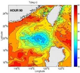 (b) | ||||||||||||||
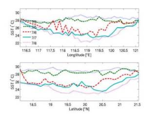
| Figure 8: (a) Horizontal SST distribution along latitude, (top) and longitude (bottom). (b) Modeled SST distribution at hour 90. | ||||||||||||||
|
The thermocline displacement due to the typhoon-induced upwelling can be evaluated using the model results. Figure 9 further shows the time series temperature profile in the upper layer (<300 m) at different locations along latitude 20.5¢XN. The temperature dropped to a depth of more than 150 m near the typhoon center (~119¢XE in Figure 8(c) after July 6. The surface mixed layer kept cooling down and reached the minima at around July 8. Since the thermocline was shallow (Figure 2) prior to the passage of typhoon Kai-Tak, the deep water appeared to be upwelled to the surface near the typhoon center. This upwelling was also associated with strong mixed layer thickening, due to enhanced mixing and entrainment. The surface mixed layer not only thickened significantly but also mixed efficiently due to strong turbulence. The thermocline became much thinner due to the upwelled thermocline in the deeper layer. This mixed layer thickening (or thermocline thinning) occurred everywhere near the strong wind stress except for the far field at 116.5¢XE (Figure 9(a)) as expected. Some previous studies have emphasized entrainment/mixing as the dominant term in the mixed layer heat budget (Jacob and Shay, 2003). Jacob et al. (2000) suggested that entrainment/mixing at the base of the mixed layer generally accounts for a large portion of the cooling (75%-90%) based on observations. Inertial oscillations were also identified from Figure 9. Based on the model results, we estimated that the thermocline upwelled from depths of 70-100 m within the areas of maximum SST change. What intensified the cooling at the center of the cold patch? The pre-conditioned shallow surface mixed layer could have played an important role. Qu et al. (2007) showed that the isothermal depth in the northern South China Sea can exceed 70 m in winter and fall below 20 m in summer near the continental slope south of China, based on the World Ocean Database 2001 (WOD01). Consistent with our observations in Figure 2, the monthly mean isothermal depth was at around 30-35 m in July where typhoon Kai-Tak hovered (Qu et al., 2007). The thermocline in that area is generally shallower during spring and summer. In the other extreme surface cooling event during the passage of typhoon Ling-Ling, the mean thermocline for the area of extreme cooling was of around 25-35 m (Qu et al., 2007). Apparently, the preconditioned shallow mixed layers contributed significantly to the extremely cool pool in both cases since the cold water below the thermocline was totally upwelled to the surface. In addition, the cooling area of typhoon Ling-Ling was also associated with a locally pre-existing cyclonic gyre from the T/P derived geopotential anomaly, which appeared to be a sub-basin scale seasonal circulation driven by the winter monsoon (Shang et al., 2008). Maximum cooling was found at the gyre center where the thermocline was much shallower than usual condition (~30 m compared to the more typical 50-100 m in winter). The pre-conditioned shallow mixed layer favored more vigorous cooling. With much cooler water nearer the surface, less energy is needed to lift the deeper water to the surface, resulting in large and rapid surface cooling. Note that typhoon Kai-Tak was declared to be a category 2 typhoon whereas typhoon Ling-Ling was classified as category 4. | ||||||||||||||
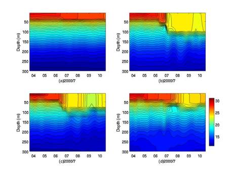 | ||||||||||||||
| Figure 9: Time-series temperature in the upper layer at different locations along latitude 20.5¢XN. (a) 116.5¢XE; (b) 118.5¢XE; (c) 119¢XE; and (d) 120.375¢XE. | ||||||||||||||
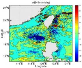 | ||||||||||||||
| Figure 10: Daily averaged vertical velocity at 45 m depth for day 5 (7/7). | ||||||||||||||
|
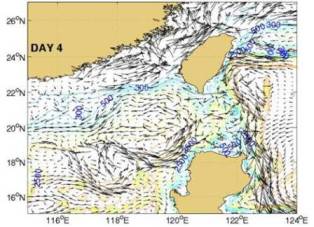
The strong upwelling during the passage of typhoon Kai-Tak should also be associated with other upwelling mechanisms, so that waters below the thermocline could be effectively upwelled to the surface. Figure 10 shows daily averaged vertical subsidence calculated at 45 m depth on July 7 (day 5); it shows strong vertical upwelling (negative subsidence is upward) near the cold pool when the typhoon hovered in the northeastern SCS. The averaged maximum vertical velocity reached 30 m/day near the typhoon center, indicating a very large amount of vertical convection. The thermocline slope in Figure 9(c) shows that the instantaneous vertical velocity can be even larger. The continuous Ekman pumping during July 5-8 due to the lingering tail of the typhoon is also enhanced by the topographical upwelling (Figure 11). Figure 11 shows the bottom currents flowing along the topography. The isobaths are also plotted in Figure 11.Very strong alongshore currents occurred near the Philippine coastal shelf. A quasi-cyclonic eddy associated with large upward motions can be observed near the center of the cold pool. This near bottom cyclonic eddy was collocated with the typhoon center, and was strengthened by the bottom bathymetry. This deep eddy, resulting from the bathymetry steering, may have enhanced the strong upwelling locally. Similar bathymetry or deep canyon enhanced upwelling can also be found in Monterey Bay, USA (e.g. Tseng et al., 2005; Tseng and Breaker, 2007). This enhancement is usually associated with strong cyclonic eddy. These features are also consistent with other earlier observations. In Hurricane Ivan (September, 2004), SSH data showed pre-existing cyclonic circulation in the areas where the extreme cooling occurred. North of the warm core eddy, maximum cooling occurred 40 to 90 km east of Ivan¡¦s track in the area of maximum SSH change. Its location agreed well with the results of Price (1981), who found that maximum cooling for rapidly moving hurricanes usually occurs 30-150 km to the right of the track. However, another maximum cooling also occurred within the area of cyclonic circulation south of the warm core eddy, closest to Ivan¡¦s track. This large cooling effect extended further west than would have been expected based on previous research. Our results suggested that the observed extreme cooling was possibly due to strong upwelling caused by the bathymetric steering. | ||||||||||||||
 (a) 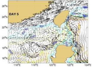 (b) | ||||||||||||||
| Figure 11: Daily averaged bottom current vectors just above the bottom cell for day 4 (a) and day 5 (b). The bathymetry is colored as contours. | ||||||||||||||
5. Summary | ||||||||||||||
In this paper, we illustrate an application of a multiple domain modeling development study using a simulation of the ocean response to typhoon Kai-Tak. An intense nonlinear mesoscale eddy was generated with a Rossby radius of O (50-100km) horizontal scale in the northeastern SCS. Inertial oscillation was clearly observed. For the first few modeled days, advection dominated as the strong wind shear drove the mixed layer flows outward, away from the typhoon center, thus forcing upwelling from deep levels with correspondingly large upwelling velocities (>30-50 m/day). The surface mixed layer deepened as the thermocline rose and caused deeper convergence. The mixed layer and thermocline merged after July 6, when the thermocline water mixed to the surface rapidly due to wind-generated turbulence. A SST drop more than 9¢XC was found in both observation and simulation. This significant SST drop resulted from the influence of a slow moving typhoon, initial stratification and bathymetry-induced upwelling in the region where the typhoon hovered. |