DieCAST ocean model

Guide for the DieCAST Ocean Model

DieCAST Home

Examples

Documentation

Mediterranean Overflow Water (MOW) simulation using a coupled multiple-grid Mediterranean Sea/North Atlantic Ocean model

Abstract

A z-level, 4th-order-accurate ocean model is applied in six two-way-coupled grids spanning the Mediterranean Sea and North Atlantic Ocean (MEDiNA). Resolutions vary from 1/4° in central North Atlantic to 1/24° in Strait of Gibraltar region.This allows the MEDiNA model to efficiently resolve small features (e.g., Strait of Gibraltar) in a multi-basin model. Such small features affect all scales because of nonlinearity and low dissipation. The grid coupling using one coarse grid overlap is nearly seamless without intergrid sponge layers. No instant convective adjustment or other highly diffusive process is used. The deep water in the 1/8° Mediterranean Sea grid is formed by the resolved flows that emulate subgrid-scale processes directly. Downslope migration of Mediterranean Overflow Water (MOW) water involves dense water flowing away from the bottom laterally over bottom stairsteps in the z-level model, thus flowing over less dense underlying water. Without excessively watermass-diluting process, the advection dominates the downslope migration of thin, dense MOW in the simulation. The model results show realistic MOW migration to the observed equilibrium depth, followed by lateral spreading near that depth. The results are also consistent with the climatology at 43°N where the MOW hugs a steep shelfslope centered at ~1 km depth. This repudiates the concept that all z-level models do poorly in density current simulations due to excessive dilution.

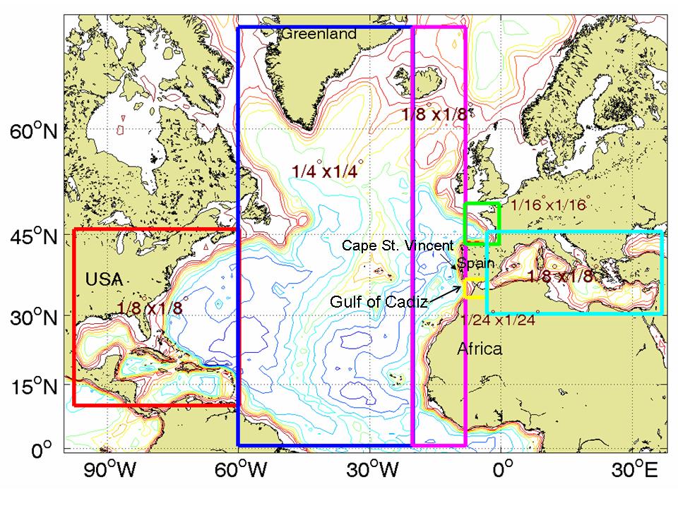Figure 1. The entire simulation domain of the six-grids MEDiNA model. The grid resolution ranges from 1/4° in the central North Atlantic Ocean grid to 1/24° in the Strait of Gibraltar regional grid. Cape St. Vincent and Gulf of Cadiz are labeled on the map.

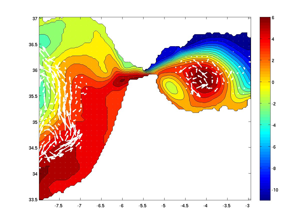Figure 2. Annual averaged sea surface height (color contours) and 1000 m depth velocity vectors in 1/24° resolution Strait of Gibraltar regional grid during year 20. The maximum velocity magnitude is 48.9 cm/s. The unit of sea surface height is cm. Longitude (°) is shown in x-axis while latitude (°) is shown in y-axis.

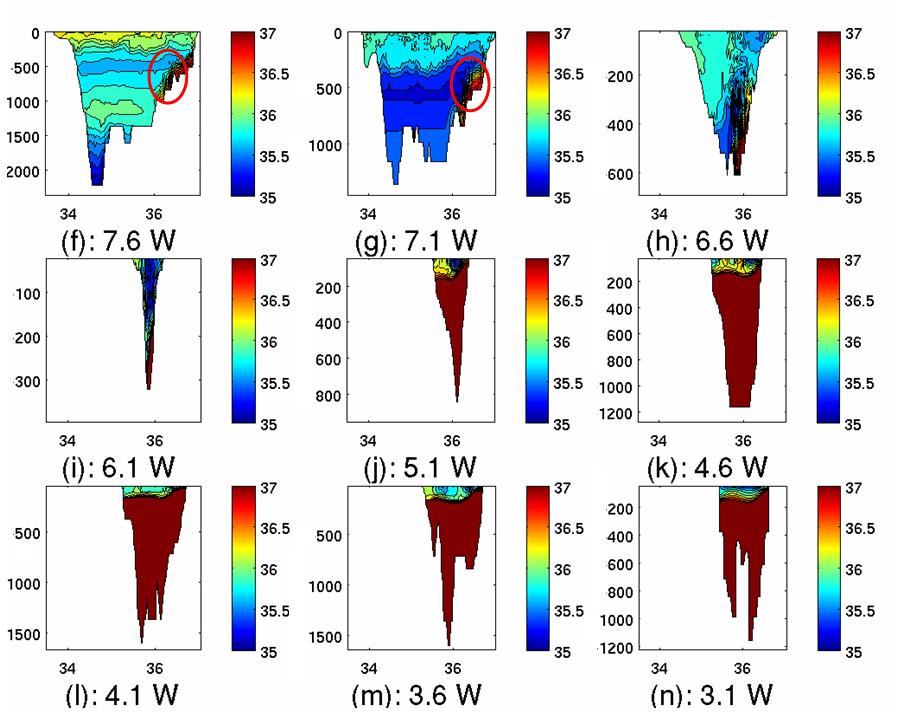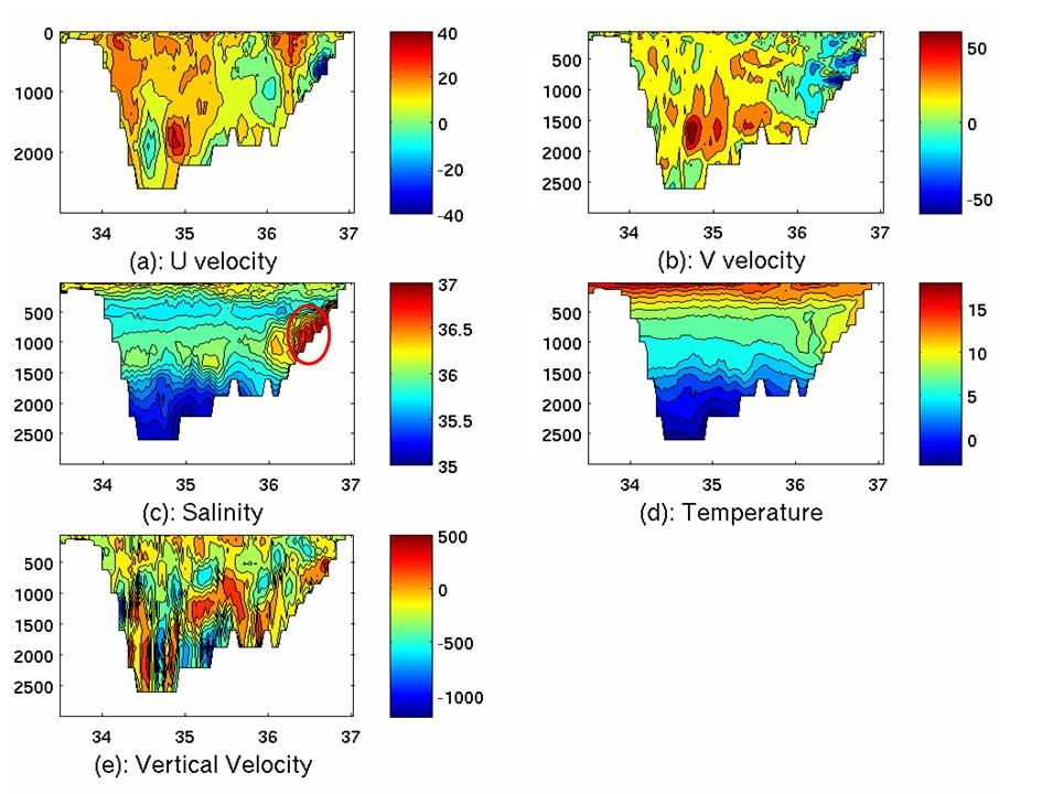
Figure 3. Vertical/latitudinal sections from the 1/24° resolution Strait of Gibraltar regional grid at the end of year 20. Panels (a)-(e) are at 8.1°W longitude, which is the model longitude adjacent to a 3-zone overlap region between the 1/8° resolution eastern North Atlantic grid and the Strait of Gibraltar regional grid (Figure 1). Panels (a)-(e) show longitudinal velocity (positive eastward), latitudinal velocity (positive northward), salinity, temperature and vertical velocity (positive downward, in m/day), respectively. Panels (f)-(n) show salinity every 1/2° going eastward from panel (c), except the extremely narrow Strait of Gibraltar choke point. 10° water is seen as deep as 1300 m. Panels (j)-(n) show the thin near-surface relatively fresh layer of North Atlantic water east of the Strait. This sequence shows the downslope MOW flow as a result of secondary flows in the bottom friction layer as one goes westward from the Strait of Gibraltar, reaching its equilibrium depth (~1000 m) in the westernmost longitude (panels (a)-(e)) where it begins its offshore spread. Dense MOW is marked as circles. Longitude (°) is shown in x-axis while depth (m) is shown in y-axis.

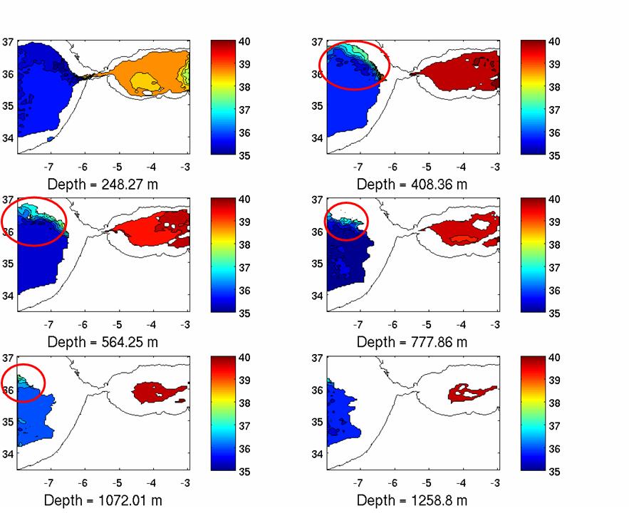Figure 4. Salinity at the end of year 20 in the 1/24° resolution Strait of Gibraltar regional grid at various depths. Dense MOW is marked as circles. The unit of color contours is g/kg. Longitude (°) is shown in x-axis while latitude (°) is shown in y-axis.

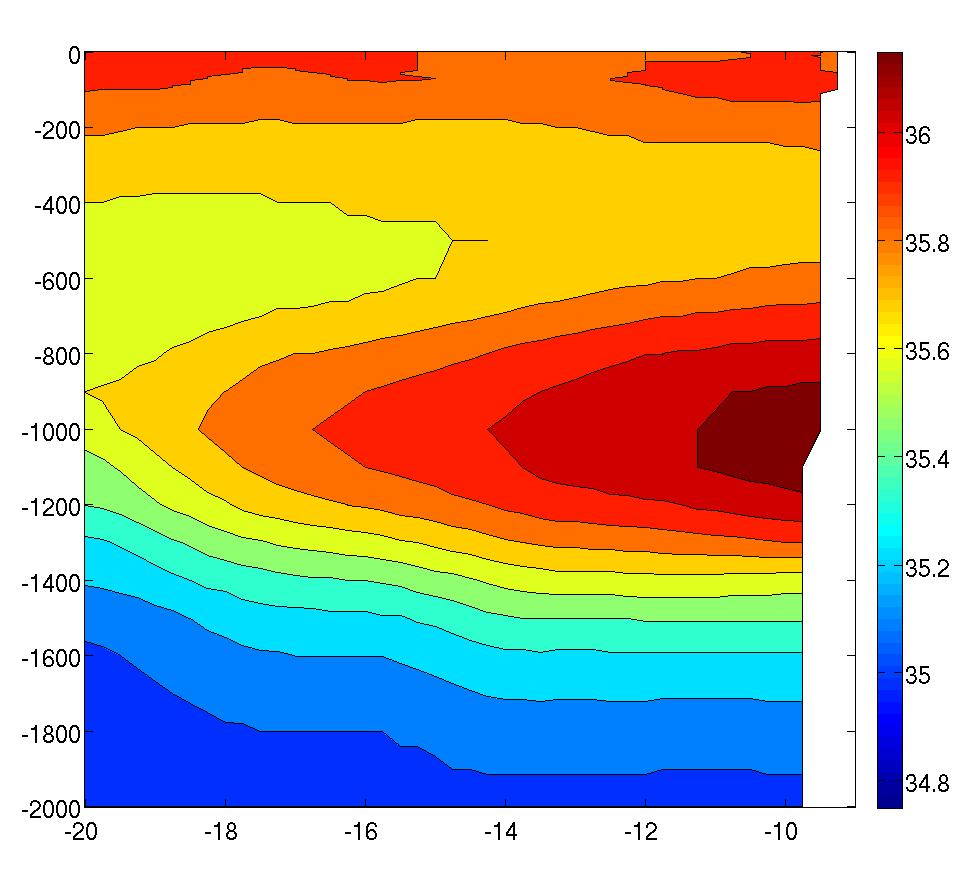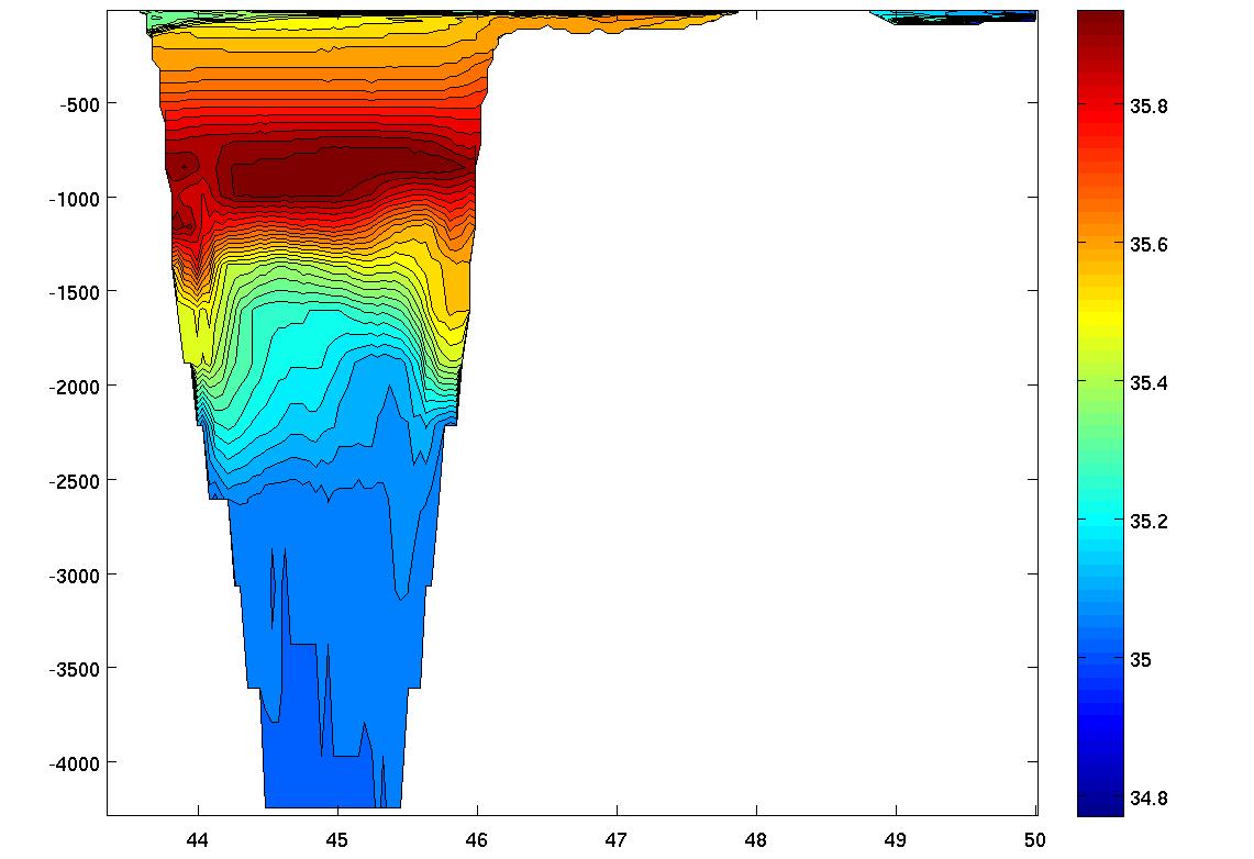
Figure 5. Vertical/longitudinal salinity section at 43°N. (a) From the annual averaged model results, showing only upper 24 model levels (scaled to compare with panel (b)) and (b) U. S. Navy’s GDEM climatology. The unit of color contours is g/kg. Longitude (°) is shown in x-axis while depth (m) is shown in y-axis.

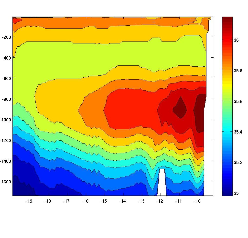
Figure 6. Annual averaged vertical/latitudinal plot of salinity in Bay of Biscay at longitude of Santander (3.8°W) shows salty MOW in intermediate depths during year 20. The Prestige oil spill in deep water off the NW corner of the Iberian Peninsula polluted its entire north coast, as consistent with this figure. Combined with Fig. 4, this indicates MOW flow path from the oil spill region to the Bay of Biscay; the same currents may entrain and transport the leaking, slowly rising oil into the Bay of Biscay. Latitude (°) is shown in x-axis while depth (m) is shown in y-axis.

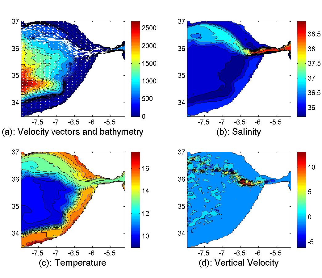Figure 7. Annual averaged deep flow west of the Strait of Gibraltar in the 1/24° resolution Gibraltar regional grid at year 20. For depth shallower (deeper) than 1075 m, time averaged bottom field (depth 1075 m horizontal field) is shown. (a) Horizontal velocity vectors and depth contours (the unit is meter); (b) Salinity; (c) Temperature; (d) Vertical velocity. Longitude (°) is shown in x-axis while latitude (°) is shown in y-axis.

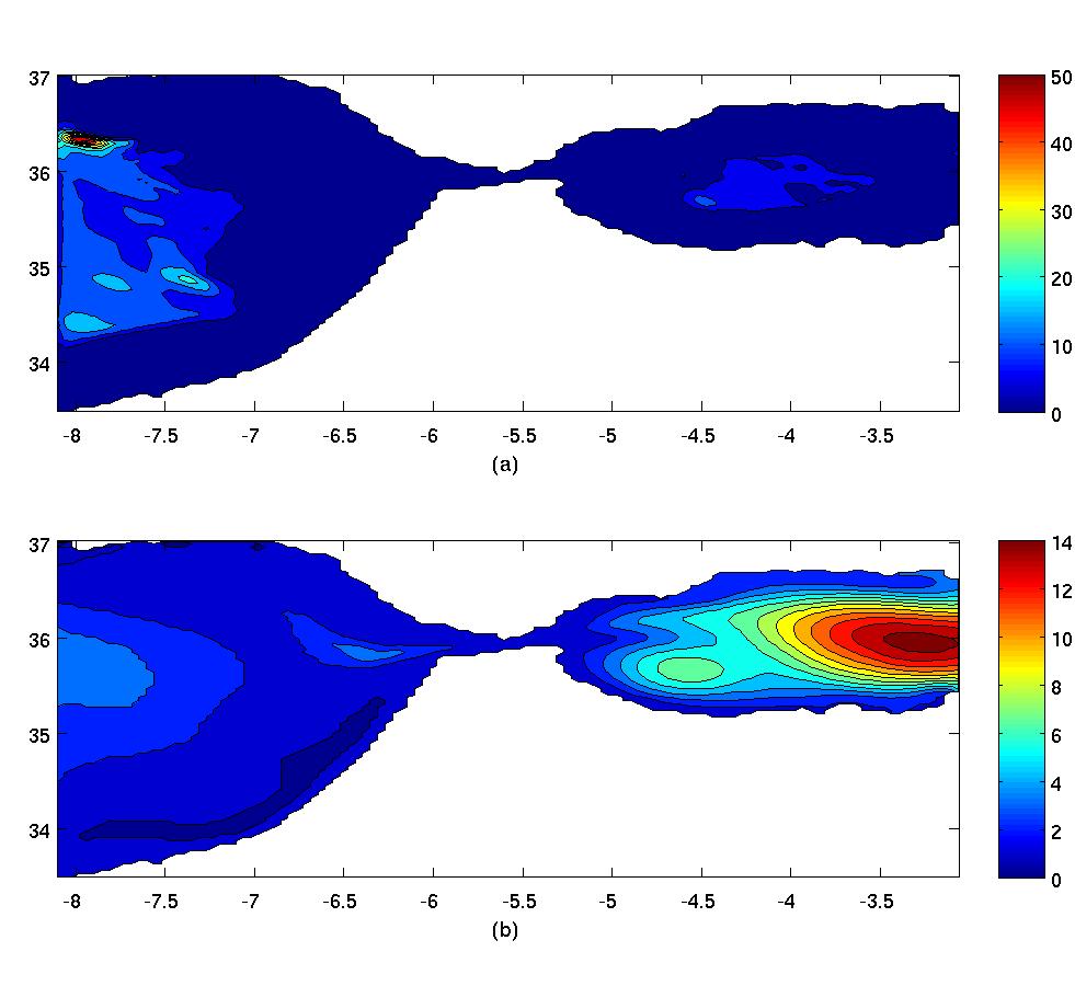Figure 8. Annual averaged eddy kinetic energy and sea surface height anomaly in the 1/24° resolution Gibraltar regional grid during year 20. (a) RMS velocity anomaly (root mean squared deviation of horizontal velocity from its time average) at 1000 m depth; bull’s eye reflects turbulent wake of MOW flow diverted around mesa-like seamount seen in Figure 6(a). The unit of color contours is cm/s. (b) RMS of sea surface height deviation from its time average; dominated by the eastward low density MAW overriding the westward MOW through the Strait of Gibraltar, and the resulting energetic western Alboran Sea anticyclonic gyres and associated cyclonic eddies. The unit of color contours is cm. Longitude (°) is shown in x-axis while latitude (°) is shown in y-axis.