| Guide for the DieCAST Ocean Model |
Nonhydrostatic simulations of the regional circulation in the Monterey Bay area
Tseng, Y. H. and Breaker, L. C. (2007), 'Nonhydrostatic simulation of the regional circulation in the Monterey Bay area', Journal of Geophysical Research-Ocean, 112, C12017, doi: 10.1029/2007JC004093.Abstract |
| The regional circulation in the vicinity of Monterey Bay is complex and highly variable. We use a one-way coupled, nonhydrostatic version of the Dietrich Center for Air Sea Technology (DieCAST) ocean model to simulate the regional circulation. Seasonally varying local wind stress, topographic irregularities, coastal upwelling, and forcing from the open ocean are all important in this region. Satellite imagery often shows a cyclonic eddy inside the bay and an anticyclonic eddy outside the bay. The offshore anticyclonic eddy is also associated with a year-round anticyclonic eddy over the Monterey Submarine Canyon (MSC). The offshore eddy is better organized during winter. It is found that the California Undercurrent (200ˇV400 m) does not enter the bay itself but is diverted offshore past the entrance of the bay, presumably to reform farther north along the coast. The main branch flows northward contributing to the deep anticyclonic eddy located approximately 50 km offshore of Monterey Bay. The simulations show aat vertical motion is greater during summer than winter, as expected. During spring upwelling, the deep waters often upwell along the walls of the canyon and then spread and mix with surrounding waters. The deep circulation enhances mixing significantly due to the topography. We further investigate the regional circulation by comparing it with the cases where the deep canyon was filled gradually. Vortex stretching over the canyon just beyond the entrance to Monterey Bay and along the adjacent continental slopes contributes to cyclonic circulation at deeper levels. Vertical sections of velocity along the axis of MSC indicate horizontal and vertical patterns of flow that are generally consistent with past observations on the circulation of Monterey Bay. |
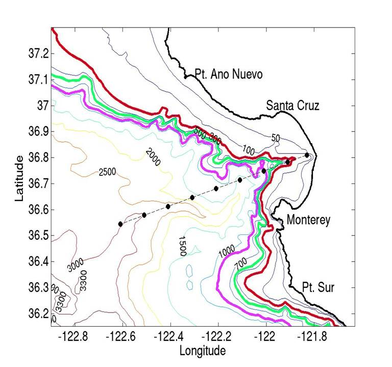 |
| Figure 1. Model domain of MBARM and bathymetry. Dashed line cuts through the Monterey Canyon. Every 20 km is shown by a black circle. The solid red, green,and pink lines represent the bathymetry at 300, 580, and 880 m depth. |
 ˇ@ |
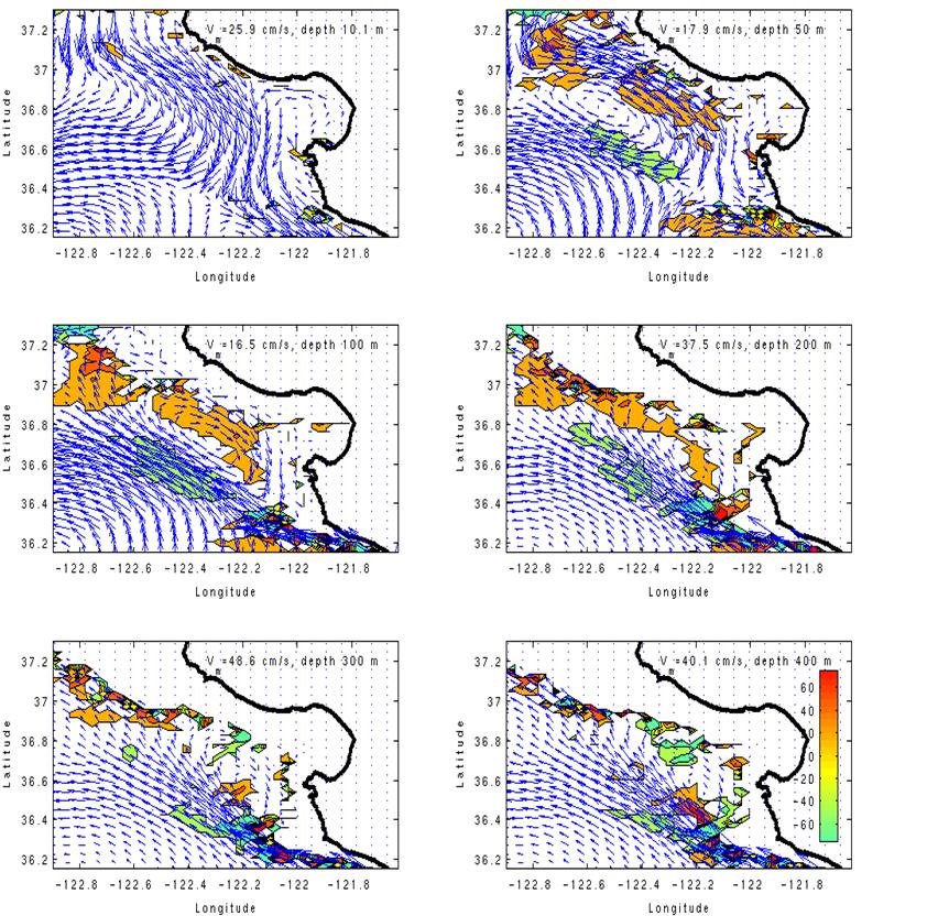
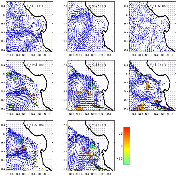
| Figure 2. Mean velocity field at various depths during summer (May to August) at depth (a) 10.1 m, (b) 50 m, (c) 100 m, (d) 200 m, (e) 300 m, and (f) 400 m. The unit of vertical velocity in the color bar is meters/week. |
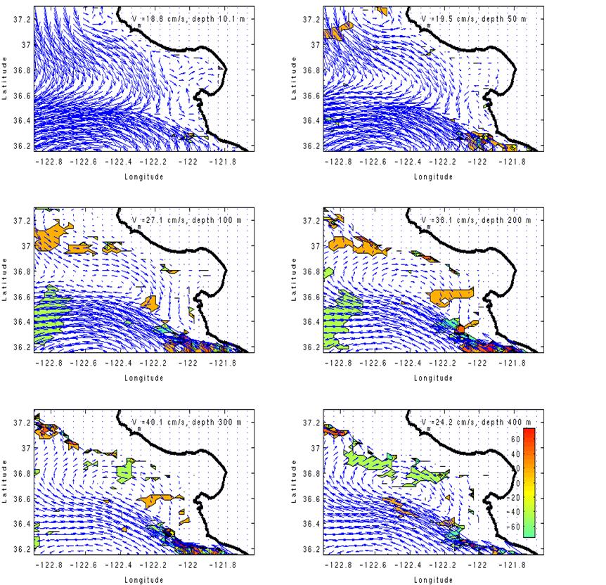 |
| Figure 3. Mean velocity field at various depths during winter (November to February) at depth (a) 10.1 m, (b) 50 m, (c) 100 m, (d) 200 m, (e) 300 m, and (f) 400 m. The unit of vertical velocity in the color bar is meters/week. |
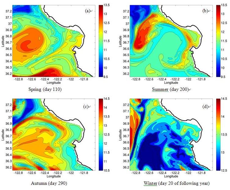 |
| Figure 4. Sea surface temperature in different seasons, with (a) spring (day 110); (b) summer (day 200); (c) autumn (day 290); (d) winter (day 20 of following year). |
 ˇ@ |
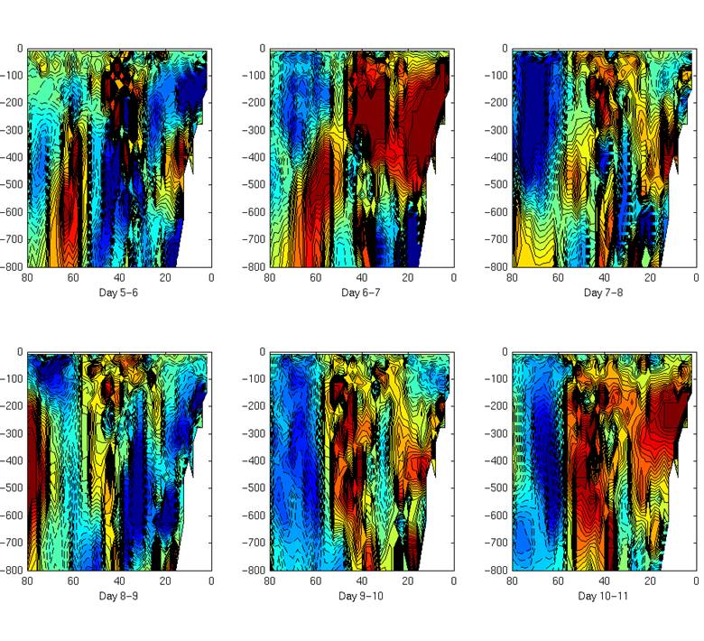
| Figure 5. Contiguous daily averaged vertical velocity along the cross
section through the center of MSC during spring upwelling starting from day 90 of year 8. Vertical velocities larger than 0.1 cm/s are marked as red while that smaller than 0.1 cm/s is marked as blue. Solid lines denote upward velocity while dash lines denote downward velocity. X-axis is the offshore distance (kilometers); y-axis is the depth (meters). The labeled day 0 corresponds to day 90 of year 8. |
|
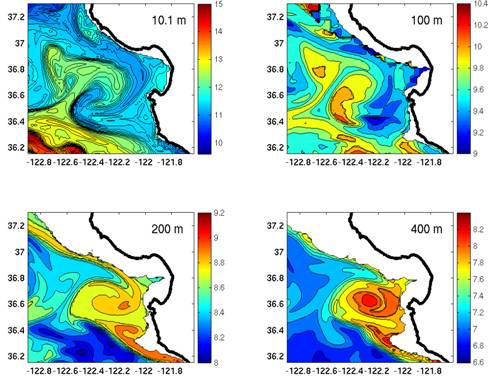
| Figure 6. Instantaneous horizontal temperature and velocity fields at several depths on day 95 of year 8. Vertical velocity is represented by the contours. |
|
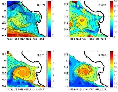
| Figure 7. Same as Figure 6 on day 100 of year 8. |
|
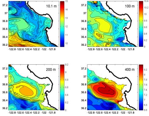
| Figure 8. Same as Figure 6 on day 105 of year 8. |
|
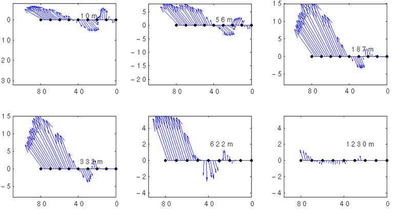
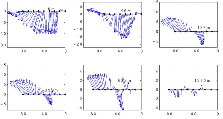
| Figure 9. The monthly averaged (taken from year 8) horizontal velocity vector in a cross-shore section cut through the center of MSC (the dash lines in Figure 1) at different depths during (a) April and (b) November. X-axis is offshore distance (kilometers). The unit in Y-axis is cm/s. |
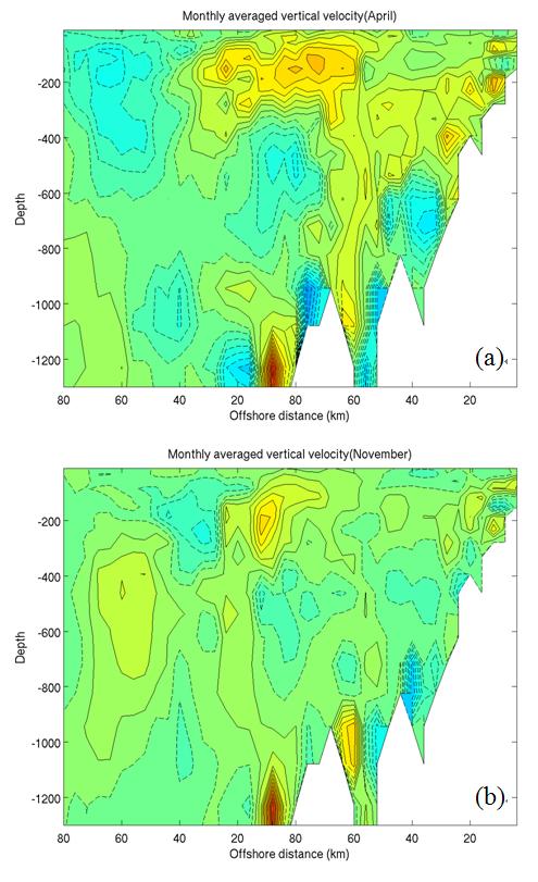 |
| Figure 10. The monthly averaged vertical velocity contours in a cross-shore section cut through the center of MSC (the dashed lines in Figure 1) at different depths (April in year 8) during (a) April and(b) November. The contours range from 0.02 cm/s to 0.02 cm/s. Solid lines denote upward velocity while dash lines denote downward velocity. |
 |
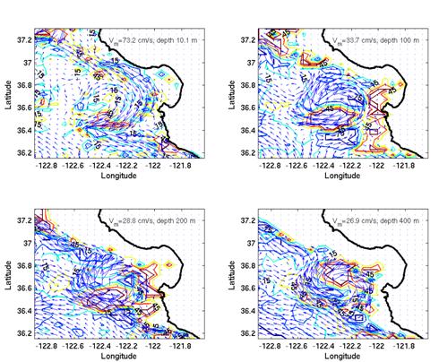
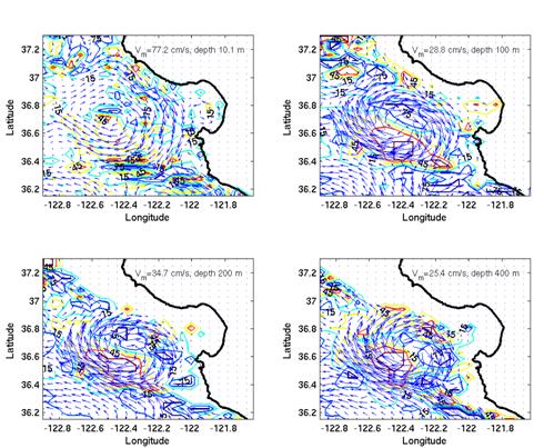
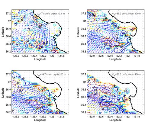
| Figure 11. The mean velocity difference between the cases "filling MSC" and "not-filling MSC" ( Vd = Vfilling MSC Vnot-filling MSC) during summer (May to August) at depth (top) 10.1 m, (middle) 200 m, and (bottom) 400 m. The topography is replaced by a flat bottom at 880 m, 580 m, and 300 m (from left to right), respectively. Vm denotes the maximum velocity difference. The color contours mark the absolute magnitude of vertical velocity greater than 5 m/week. The unit of vertical velocity in the color bar is meters/week. |
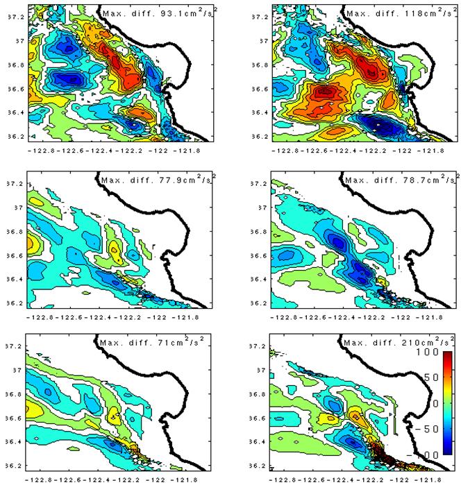 |
| Figure 12. Same as Figure 11 during winter (November to February). |
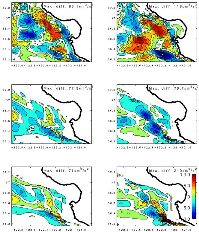 |
| Figure 13. Comparison of the total kinetic energy difference between the
cases "filling" and"notfilling" MSC during summer at depth (top) 10.1 m, (middle) 200 m, and (bottom) 400 m. The topography is replaced by a flat bottom at (left) 880 m and (right) 580 m, respectively. The color contours mark the absolute magnitude greater than 5 cm2/s2. The color bar has unit cm2/s2. |
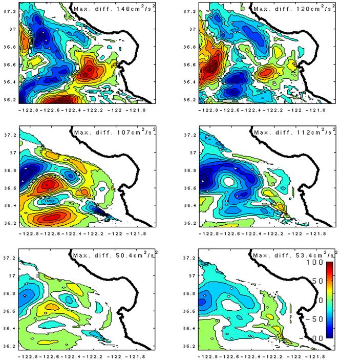 |
| Figure 14. Same as Figure 13 during winter. |
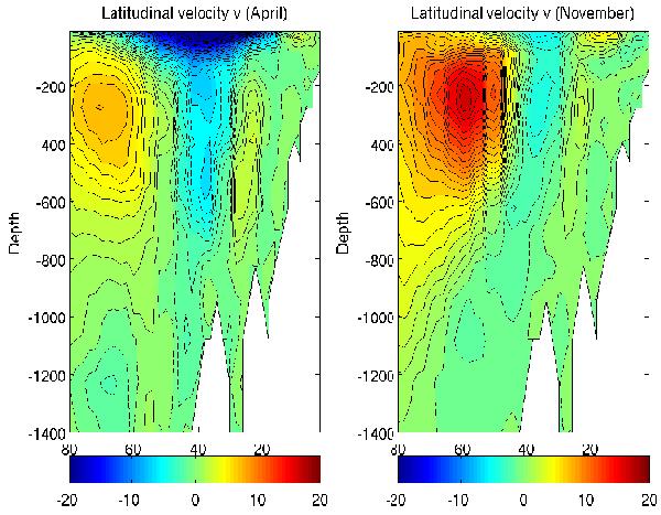 |
| Figure 15. Comparison of the monthly averaged vertical sections in April and November for the latitudinal "v") component of velocity from the surface to 1400 m along the axis of MSC (see Figure 1). |