Numerical Methods

TIMCOM is an efficient and accurate model using the second-order Leap-frog temporal scheme with fourth-order spatial approximation. Furthermore, the modified Robert-Asselin filter is employed to eliminate the time splitting issue. The model domain is discretized by a set of resolution parameters, i.e. I0, J0, and K0 along the horizontal and vertical directions with the grid index i, j, and k, respectively. A non-uniform grid spacing can be set (the non-uniform vertical layers). For variable arrangement, TIMCOM uses a blend of collocated and staggered grids structures (Arakawa A and C grids). The cell-averaged variables ui,j,k, vi,j,k, Si,j,k, Ti,j,k, pi,j,k, and ρi,j,k are defined at the cell center (i, j, k), while the face-averaged velocity components Ui+1/2,j,k, Vi,j+1/2,k, and Wi,j,k+1/2 are located on the faces (i+1/2, j, k), (i, j+1/2, k), and (i, j, k+1/2). Note that ρi,j,k in the model represents density variations ρ′, which is a small deviation from the mean reference value ρ0, i.e. ρ′=ρ−ρ0. As a consequence, pi,j,k indicates pressure perturbations, rather than the total pressures.


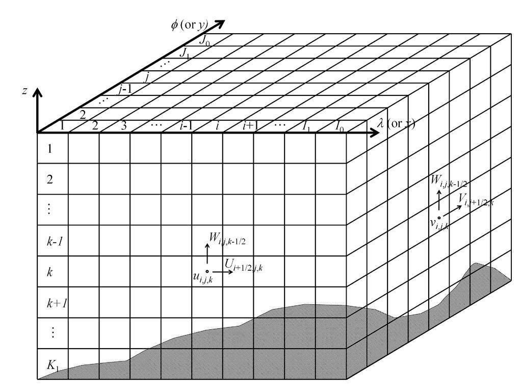
Figure N.1: computational grids in TIMCOM.


The overall numerical algorithm of TIMCOM can be divided into three major steps: (i) update intermediate flow field through horizontal momentum equations as well as conservation equations at the time step n; (ii) substitute the intermediate velocities and corrections into the conservative continuity equation and solve the resulting 2D Poisson equation for pressure adjustment. Then, the final flow field can be readily determined; (iii) apply modified Robert-Asselin filter to the flow variables and advance to the time step n+1. Each step is further explained in the following.
In the first step, we discretize the horizontal momentum equation to calculate the intermediate longitudinal-direction velocity ~un+1, i.e.
~
u
 
n+1
i,j,k 
−un−1i,j,k

2∆t
=
Lun 1

ρ0R cosϕ
∂(pn−1s+ pnb)

∂λ
+Dm un−1 +

∂z
[Au

∂z
(un−1) ],
(N.1)
where
L un
=
Uni+1/2,j,kuni+1/2,j,k−Uni−1/2,j,kuni−1/2,j,k

R cosϕ∆λi
(N.2)
+
Vni,j+1/2,kuni,j+1/2,k−Vni,j−1/2,kuni,j−1/2,k

R ∆ϕj
(N.3)
+
Wni,j,k+1/2uni,j,k+1/2−Wni,j,k−1/2uni,j,k−1/2

∆zk
,
(N.4)


∂λ
[pn−1(n)s(b)]
=
pn−1(n)i−2,j,k−8pn−1(n)i−1,j,k+8pn−1(n)i+1,j,k−pn−1(n)i+2,j,k

12 ∆λi
,
(N.5)

Dmun−1
=
Am

R2
( un−1i+1,j,k−2un−1i,j,k+un−1i−1,j,k

cos2 ϕ∆λi
+ un−1i,j+1,k−2un−1i,j,k+un−1i,j−1,k

∆ϕj
(N.6)
+
tanϕ un−1i,j+1,k−un−1i,j−1,k

2∆ϕi
) ,
(N.7)


∂z
[Au

∂z
(un−1) ]
=
1

∆zk
[ (Au)i,j,k ui,j,k+1n−1−ui,j,kn−1

∆zk
−(Au)i,j,k−1 ui,j,kn−1−ui,j,k−1n−1

∆zk
],
(N.8)
in which the vertical eddy viscosity Au is determined by the approach of Pacanowski & Philander (1981) (see here). Similar procedure can be directly applied to obtain the intermediate latitudinal-direction velocity ~vn+1, final potential temperature Tn+1 and salinity Sn+1. The intermediate velocities are further updated to involve the Coriolis effects, i.e.
^
u
 
n+1
 
=
~
u
 
n+1
 
+2∆t
~
F
 
(
^
v
 
n+1
 
+vn−1

2
) =
~
u
 
n+1
 
+
~
F
 
∆t vn−1 +
~
F
 
∆t
^
v
 
n+1
 
,
(N.9)
^
v
 
n+1
 
=
~
v
 
n+1
 
−2∆t
~
F
 
(
^
u
 
n+1
 
+un−1

2
) =
~
v
 
n+1
 
~
F
 
∆t un−1
~
F
 
∆t
^
u
 
n+1
 
,
(N.10)
where ~F ≡ f+[(untanϕ)/R]. Solving equations (N.9) and (N.10) gives
^
u
 
n+1
 
= 1

1+(
~
F
 
∆t)2
(
^
u
 
n+1
* 
+
~
F
 
∆t ·
^
v
 
n+1
* 
),
(N.11)
^
v
 
n+1
 
= 1

1+(
~
F
 
∆t)2
(
^
v
 
n+1
* 
~
F
 
∆t ·
^
u
 
n+1
* 
),
(N.12)
where
^
u
 
n+1
* 
=
~
u
 
n+1
 
+
~
F
 
∆t ·vn−1,
(N.13)
^
v
 
n+1
* 
=
~
v
 
n+1
 
~
F
 
∆t ·un−1.
(N.14)
For the face-averaged velocity field, the fourth-order interpolation is employed. The intermediate face velocity is given by
^
U
 
n+1
i+1/2,j,k 
=
^
u
 
n+1
i−1,j,k 
+7
^
u
 
n+1
i,j,k 
+7
^
u
 
n+1
i+1,j,k 
^
u
 
n+1
i+2,j,k 

12
.
(N.15)
The second step is to determine the final velocity field. The basic idea is that correct the intermediate velocities to achieve an appropriate pressure formulation, i.e. psn rather than psn−1 used in equation. Thus, the final face velocities can be written as
Un+1i+1/2,j,k =
^
U
 
n+1
i+1/2,j,k 
+ δUn+1i+1/2,j,k,
(N.16)
Vn+1i,j+1/2,k =
^
V
 
n+1
i,j+1/2,k 
+ δVn+1i,j+1/2,k,
(N.17)
where
δUn+1i+1/2,j,k
=
2 ∆t

ρ0Rcosϕ

∂λ
(psn−psn−1) = − 2 ∆t

ρ0Rcosϕ

∂λ
(δpsn),
(N.18)
δVn+1i,j+1/2,k
=
2 ∆t

ρ0R

∂ϕ
(psn−psn−1) = − 2 ∆t

ρ0R

∂ϕ
(δpsn) .
(N.19)
Substituting equations (N.16)-(N.19) into the conservative continuity equation results in the 2D Poisson equation for pressure adjustment δpsn, i.e.
2∆t

ρ0R2 cosϕ

0

−h 
[

∂λ
1

cosϕ
∂δpns

∂λ
+

∂ϕ
( ∂δpns

∂ϕ
) cosϕ] dz =
^
w
 
n+1
−h 
,
(N.20)
where the last term is a convenient shorthand notation and can be expressed as
^
w
 
n+1
−h 
= 1

R cosϕ
(

∂λ

0

−h 
^
U
 
n+1
 
dz+

∂ϕ

0

−h 
^
V
 
n+1
 
cosϕdz).
(N.21)
The system equation (N.20) can be solved by an efficient error vector propagation (EVP) elliptic solver. Once the pressure adjustment δpns is determined, the corrections for the face-averaged velocities δUn+1i+1/2,j,k and δVn+1i,j+1/2,k can be directly obtained by equations (N.18)-(N.19). Further, interpolate the velocity corrections back to the collocated point (i, j, k), giving the changes for the final cell-averaged velocities, e.g.
un+1i,j,k =
^
u
 
n+1
i,j,k 
+ δun+1i,j,k,
(N.22)
where
δun+1i,j,k = −δUn+1i−3/2,j,k+13δUn+1i−1/2,j,k+13δUn+1i+1/2,j,k−δUn+1i+3/2,j,k

24
.
(N.23)
The flow variables un+1, vn+1, Un+1, Vn+1, and pns are fully updated by velocity corrections and pressure adjustment. Vertical velocity Wn+1 is calculated using continuity equation.
In the last step, the modified Robert-Asselin filter is applied. Recognizing that the Leap-frog temporal scheme is widely used in many general circulation models, proposed a modified filter to resolve the time slitting issue. In contrast to the standard Robert-Asselin filter, the modified version provides third-order accuracy for amplitude errors. The filtered velocities for the next time step t = t + ∆t are
un−1i,j,k|t=t+∆t
=
[uni,j,k + υα

2
(un−1i,j,k−2uni,j,k+un+1i,j,k)]|t=t,
(N.24)
uni,j,k|t=t+∆t
=
[un+1i,j,k υ(1−α)

2
(un−1i,j,k−2uni,j,k+un+1i,j,k)]|t=t,
(N.25)
where 0 ≤ υ ≤ 1 and 0 ≤ α ≤ 1 are two filter parameters controlling the family of the modified Robert-Asselin-filtered Leap-frog scheme (denoted as MRAF). Note that the special case υ = 0 leads to the classic (non-filtered) Leap-frog scheme (denoted as NONF) while the case α = 1 results in the standard Robert-Asselin-filtered Leap-frog scheme (denoted as SRAF).

Go Back to Model Description


Copyright ©2011 The TIMCOM Development Group
Home | License | Contact Us