Vertical Grid Spacing

Vertical Grid Spacing

For ocean circulation modelling, a finer grid resolution is usually needed at upper layers to accurately resolve the complicated vertical structure of flow field or near the bottom to well represent the topography. The uniform vertical grid spacing (see Fig. Z.1(a) ) can be easily used to discretize the computational domain. However, the computation can be relatively expensive due to the large number of grids in the whole water column while a sufficiently high resolution is employed to capture detailed flow features. In contrast, nonuniform vertical grid spacing is an effective alternative to achieve the required accuracy with a reasonable computational expense. TIMCOM provides three different types of nonuniform grids, generating (i) linear-exponential stretched, (ii) power stretched, and (iii) user-defined vertical layers. Their corresponding values of the option flag ZOP are 1, 2, and 3, respectively. In the following, we briefly describe the vertical grid generation.

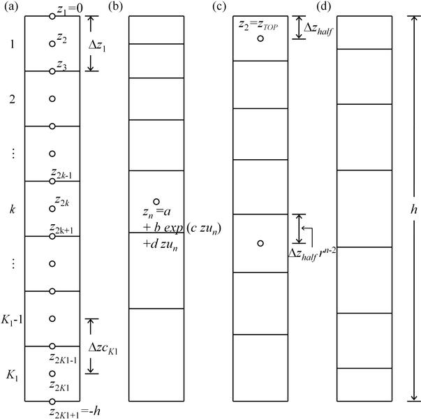
Figure Z.1: (a) uniform, (b) linear-exponential stretched, (c) power stretched, and (d) user-defined vertical layers.

a) Vertical Grid Generation

In the model, K₁ (or K₀-1) vertical grids are generated by specifying the information of z levels, rather than the thickness of each layer. The z levels of the cell center and its bounded interfaces at layer k are denoted as z_2k, z_2k−1, and z_2k+1, respectively. Once the z levels are created, the model further calculates the distances between grid lines/centers and saves them in an inverse form for later computation.

1/∆z_k=1/(z_2k+1−z_2k−1) , k=1,2, …K1

1/∆zc_k=1/(z_2k−z_2k−2) , k=2,3, …K1
b) Linear-Exponential Stretched Vertical Layers (ZOP = 1)

Generally, an exponential stretching is employed in the z direction, concentrating vertical cells near surface (see Fig. Z.1(b)). In the model, a combination of linear and exponential functions is used to determine the z levels including the interfaces (odd indexes) and cell centers (even ones), i.e.

z_n = a + b·exp[−c(n−1)([(−h)/(2K₁)])] + d(n−1)([(−h)/(2K₁)]) , n=1,2, …, 2K₁, 2K₁+1
or

z_n = a + b·exp[−c·zu_n] + d·zu_n , n=1,2, …, 2K₁, 2K₁+1

where n is the index of z-level array with z₁=0 (or z_2K₁+1=−h) at the surface (or bottom); a=−(1−d)h/[1−exp(ch)]; b=−a; c and d are the user-specified parameters; h is the maximum water depth; and zu_n represents the uniform distributed z levels.

c) Power Stretched Vertical Layers (ZOP = 2)

Vertical stretching along the z direction can be determined by the power law as well. The users need to specify the z level of the top-layer cell z₂=−z_TOP, giving the half thickness of the top layer ∆z_half=z₁−z₂=z_TOP. As the depth gets deeper, the lower grids are stretched (or contracted) by a grid stretching ratio r, which will be determined in the program. The power stretched vertical layers (see Fig Z.1(c)) can be expressed as

z_n=z_n−1−∆z_half ·r⁽ⁿ⁻²⁾, n=3,4,…, 2K₁, 2K₁+1

d) User-Defined Vertical Layers (ZOP = 3)

The users can also define any arbitrary vertical layers (as shown in Fig Z.1(d) ) through the z-level data in the file Z_CUSTOM_CASENAME.TXT. We should note that the data array with a length of 2K₁+1 would be required for K₁ layers and odd/even indexes represent the interfaces/cell centers.

Go Back to Numerical Methods